Chapter 5: Advanced Querying
Introduction
In this chapter, we will delve into advanced querying techniques that will enhance your ability to retrieve and manipulate data from multiple tables. We will cover topics such as joining tables using different types of joins, aggregating data with GROUP BY and HAVING, utilizing subqueries and nested queries, and leveraging common table expressions (CTEs).
5.1 Joining Multiple Tables Using Different Types of Joins
When working with relational databases, it is common to have data distributed across multiple tables. Joining tables allows you to combine related data from different tables into a single result set. We will explore various types of joins, including:
Inner Join: Retrieves rows that have matching values in both tables being joined.
Left Join: Retrieves all rows from the left table and the matching rows from the right table, if any.
Right Join: Retrieves all rows from the right table and the matching rows from the left table, if any.
Full Join: Retrieves all rows from both tables, including unmatched rows.
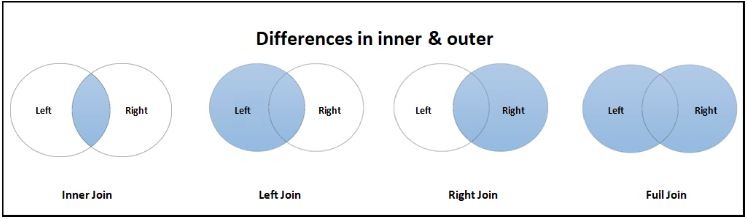
Joins in SQL can be visualized using Venn diagrams, which provide a graphical representation of the relationships between tables. Here's an explanation of joins in terms of Venn diagrams:
Inner Join: An inner join returns the intersection of the tables involved, including only the matching records. In a Venn diagram, an inner join can be represented by the overlapping region between two circles, where the overlapping area represents the common records.
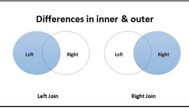
Left Join: A left join returns all records from the left table (Customers) and the matching records from the right table (Orders). In a Venn diagram, a left join can be represented by the left circle, including the overlapping region with the right circle.
Right Join: A right join returns all records from the right table (Orders) and the matching records from the left table (Customers). In a Venn diagram, a right join can be represented by the right circle, including the overlapping region with the left circle.
Full Join: A full join returns all records from both tables, including both the matching and non-matching records. In a Venn diagram, a full join can be represented by the overlapping region between two circles, including the non-overlapping areas of each circle.
By visualizing joins using Venn diagrams, you can better understand how the records from different tables are combined based on the join conditions. This graphical representation helps in grasping the concept of joins and provides a visual aid for understanding the resulting data sets.
Let's consider an example:
sqlCopy code
SELECT customers.customer_id, customers.name, orders.order_id, orders.order_date FROM customers INNER JOIN orders ON customers.customer_id = orders.customer_id;
In this example, we use an inner join to combine the "customers" and "orders" tables based on the customer_id column. The result set will contain only the rows where there is a match in both tables.
Structure of Inner Join
SELECT
T1.Field1,
T1.Field2,
T2.Field1,
T2.Field2
FROM
Table 1 as T1
INNER JOIN
Table 2 s T2
ON
T1.Field1 = T2.Field1;
Few more SQL Query code Example of LEFT JOIN , RIGHT JOIN and FULL Join are s below,
LEFT JOIN
SELECT Customers.customer_id, Customers.name, Orders.order_id, Orders.order_date
FROM Customers
LEFT JOIN Orders ON Customers.customer_id = Orders.customer_id;
RIGHT JOIN
SELECT Customers.customer_id, Customers.name, Orders.order_id, Orders.order_date
FROM Customers
RIGHT JOIN Orders ON Customers.customer_id = Orders.customer_id;
FULL JOIN
SELECT Customers.customer_id, Customers.name, Orders.order_id, Orders.order_date
FROM Customers
FULL JOIN Orders ON Customers.customer_id = Orders.customer_id;
5.2 Aggregating Data with GROUP BY and HAVING
Aggregation functions, such as SUM, AVG, COUNT, MIN, and MAX, allow us to perform calculations on a group of rows. The GROUP BY clause is used to group the rows based on one or more columns, while the HAVING clause allows us to filter the groups based on specific conditions. Consider the following example:
sqlCopy code
SELECT category, COUNT(*) AS total_products FROM products GROUP BY category HAVING COUNT(*) > 5;
In this example, we calculate the total number of products in each category and filter out the groups that have more than 5 products. The result will display the category and the corresponding count of products.
5.3 Subqueries and Nested Queries
Subqueries, also known as nested queries, are queries that are embedded within other queries. They allow us to retrieve data based on the results of another query. Here's an example:
sqlCopy code
SELECT product_name, price FROM products WHERE price > (SELECT AVG(price) FROM products);
In this example, the subquery calculates the average price of all products, and the main query retrieves products with a price greater than the average.
We will explore more complex subquery scenarios, such as using subqueries in the SELECT, FROM, and HAVING clauses, as well as correlated subqueries.
5.4 Common Table Expressions (CTEs)
Common table expressions (CTEs) provide a way to create temporary result sets that can be used within a query. They enhance readability and maintainability by breaking down complex queries into smaller, more manageable parts. Here's an example:
sqlCopy code
WITH top_customers AS ( SELECT customer_id, SUM(order_total) AS total_spent FROM orders GROUP BY customer_id HAVING SUM(order_total) > 1000 ) SELECT customers.name, top_customers.total_spent FROM customers INNER JOIN top_customers ON customers.customer_id = top_customers.customer_id;
In this example, the CTE "top_customers" calculates the total amount spent by each customer and filters out the customers who have spent more than 1000. The main query joins the CTE with the "customers" table to retrieve the customer names and their total spending.
Throughout this chapter, we have provided detailed explanations and numerous examples to guide you through advanced querying techniques. By practicing these examples and experimenting with different scenarios, you will gain a solid understanding of joining tables, aggregating data, working with subqueries, and utilizing common table expressions.
In the next chapter, we will focus on data manipulation language (DML), which involves modifying data in the database through INSERT, UPDATE, and DELETE operations.